Estimating a population mean
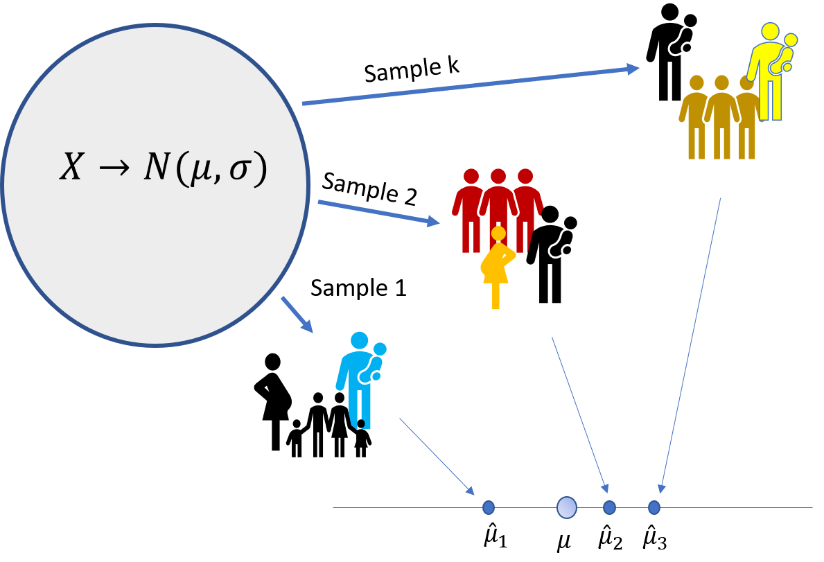
A population mean \(\mu\) can be estimated from appropriate sampling the population. As each sample will produce a different result, we need some sort of procedure for dealing with the uncertainty of the result. Confidence intervals are these tools.
Conficence interval (CI) for a population mean
The \((1-\alpha)\) CI for a population mean is computed as: \(\mu \rightarrow m \pm t_{1-\alpha/2,n-1} \times \frac{s}{\sqrt{n}}\) where \(m\) is the sample mean and \(s\) the sample standard deviation. The sample size \(n\) indicates how many individuals have been included in the sample.Exercises in this application
- Explore the distribution of the means of different samples
- Estimate a population mean from data
- Perform simulations to compare the CI of different samples when estimating a population mean
- Estimate the difference of the means of two populations
- Compute the required sample sizes for obtaining precise estimations
Parameter estimation by maximum likelihood
The method of maximum likelihood gives estimators that maximize the likelihhod function. In can be interpreted as estimating the paramters that makes it more like to have obtained the sample. For a normal variable, the likelihood function is: $$L=\prod_{i=1}^n \left(\frac{1}{\sigma \sqrt{2/\pi}} e^{-\frac{(x_i-\mu)^2}{2\sigma^2}}\right)$$ The maximum likelihood estimators of \(\mu\) and \(\sigma\) are: $$\hat \mu = \frac{\sum\limits_{i=1}^n x_i}{n}$$ $$\hat \sigma = \frac{\sum\limits_{i=1}^n (x_i-\hat \mu)^2}{n-1}$$
Maximum likelihood estimates
Contour of likelihood values as a function of \(\mu\) and \(\sigma\).
The red point indicates the actual parameters.
The black points indicates the ML estimates.
95% prediction intervals
\( X \rightarrow \mu \pm z_{1-\alpha/2} \sigma\) \(\bar X \rightarrow \mu \pm z_{1-\alpha/2} \frac{\sigma}{\sqrt{n}}\) \(z_{1-\alpha/2}=1.96\)
Estimate the mean from a sample
\(\mu \rightarrow m \pm t_{1-\alpha/2,n-1} \times \frac{s}{\sqrt{n}}\)
The required computations are:
Results
Result
$$\mu \rightarrow m \pm t_{1-\alpha/2,n-1} \times \frac{s}{\sqrt{n}}$$
In a practical case, we are interested in obtaining precise CI. This precission depends dramatically on the sample size. Here you can compute the required sample size for obtaining the desired precission, given a previous knowledge of the approximated value of the standard deviation.
The required sample size for a \((1-\alpha)\) IC with precission \(\delta\) is computed as: $$n \rightarrow z_{1-\alpha/2}^2 \frac{\hat \sigma^2}{\delta ^2}$$ where \(\hat \sigma \approx s\)
Required sample size for different \(\delta\) values
You can set a theoretical distribution \(N(\mu,\sigma)\) and obtain a number of samples with a given sample size. The application computes the corresponding CI for \(\mu\) and compares the results for the different samples. According to the definition of CI, 95% of the computed results will include the true value of the population parameter.
Population values
Results
One of the most basic experimental designs compares the results of a control group and a treatment group. This is done by estimating the difference of the population means. The same procedure could be used to compare a biomarker among two populations. In this exercise we provide simulations for understanding the interpretation of the CI for the difference of two population means.
Sample 1
Sample 2
The \((1-\alpha)\) confidence interval for the diffence of two means is computed as: $$\bar X_1-\bar X_2 \pm t_{1-\alpha/2,\nu} \sqrt{\frac{s_1^2}{n_1}+\frac{s_2^2}{n_2}} $$ Assuming large samples, the precission of the CI can be written as: $$\delta=z_{1-\alpha/2} \sqrt{\frac{s_1^2}{n_1}+\frac{s_2^2}{n_2}}$$ If we call \(r=(n_2/n_1) \rightarrow n_2=r \times n_1\). Then: $$n_1=z_{1-\alpha/2}^2 \frac{r \times s_1^2 + s_2^2}{r \times \delta^2}$$
You can define the parameters of two populations and obtain samples for estimating the difference \(\mu_1-\mu_2\). You can also fix the minimum difference for considering a relevant effect for that difference.
You can define the parameters of two populations and obtain samples for estimating the difference \(\mu_1-\mu_2\). The blue line indicates the actual value of the difference of menas defined by the user. The red line indicates the null hypothesis that population means are equal. Try to figure out which is the effect of sample size in providing enough information for identifying the true differecne of means.
Concers on misusing intervals
It is important to understand the difference between various types of intervals. Here, we compare them in a sample of two groups
Interpretation of different intervals
We assume that the studied variable is distribruted as a \(N(\mu_i,\sigma_i)\) in each group \(i\). We can obtain two classes of intervals:
Confidence intervals: Approximate regions that would include the value of the population parameter
Definitions
Population mean (\(\mu\)): Is a parameter of the distribution.
Population standard deviation: (\(\sigma\)): Is a parameter of the distribution.
Population standard error of the mean: (\(\frac{\sigma}{\sqrt{n}}\)): Is a parameter of the distribution.
Sample size (n): The number of observations in the sample. Sample mean (m): Is an estimation of the population mean (\(\mu\))
Sample standard deviation (s): Is an estimation of the population standard deviations (\(\sigma\))
Sample standard error of mean (sem:\(\frac{s}{\sqrt{n}}\)): Is an estimation of the population error of mean
Reference intervals
\(\mu \pm \sigma \): This interval is where we expect to observe an approximated 68% of the values in a sample of any size.
\(\mu \pm 1.96 \times \sigma \): This interval is where we expect to observe an approximated 95% of the values in a sample of any size.
\(m \pm s \): This interval is an estimation of the reference interval where we expect to observe an approximated 68% of the values in a sample of any size.
\(m \pm 1.96 \times s \): This interval is an estimation of the reference interval where we expect to observe an approximated 95% of the values in a sample of any size.
Confidence intervals
\(m \pm sem\) is an approximated 68% confidence interval for \(\mu\) in large samples
\(m \pm 1.96 \times sem\) is an approximated 95% confidence interval for \(\mu\) in large samples
\(m \pm t_{n-1,1-\alpha/2} \times sem\) is an approximated \((1-\alpha)\) confidence interval for \(\mu\).